LaTeX research paper template
A LaTeX research paper template for a preprint or any paper whose venue has no class of its own.
- Engine: pdfLaTeX
- Bibliography: BibTeX
- License: Public domain, use freely.
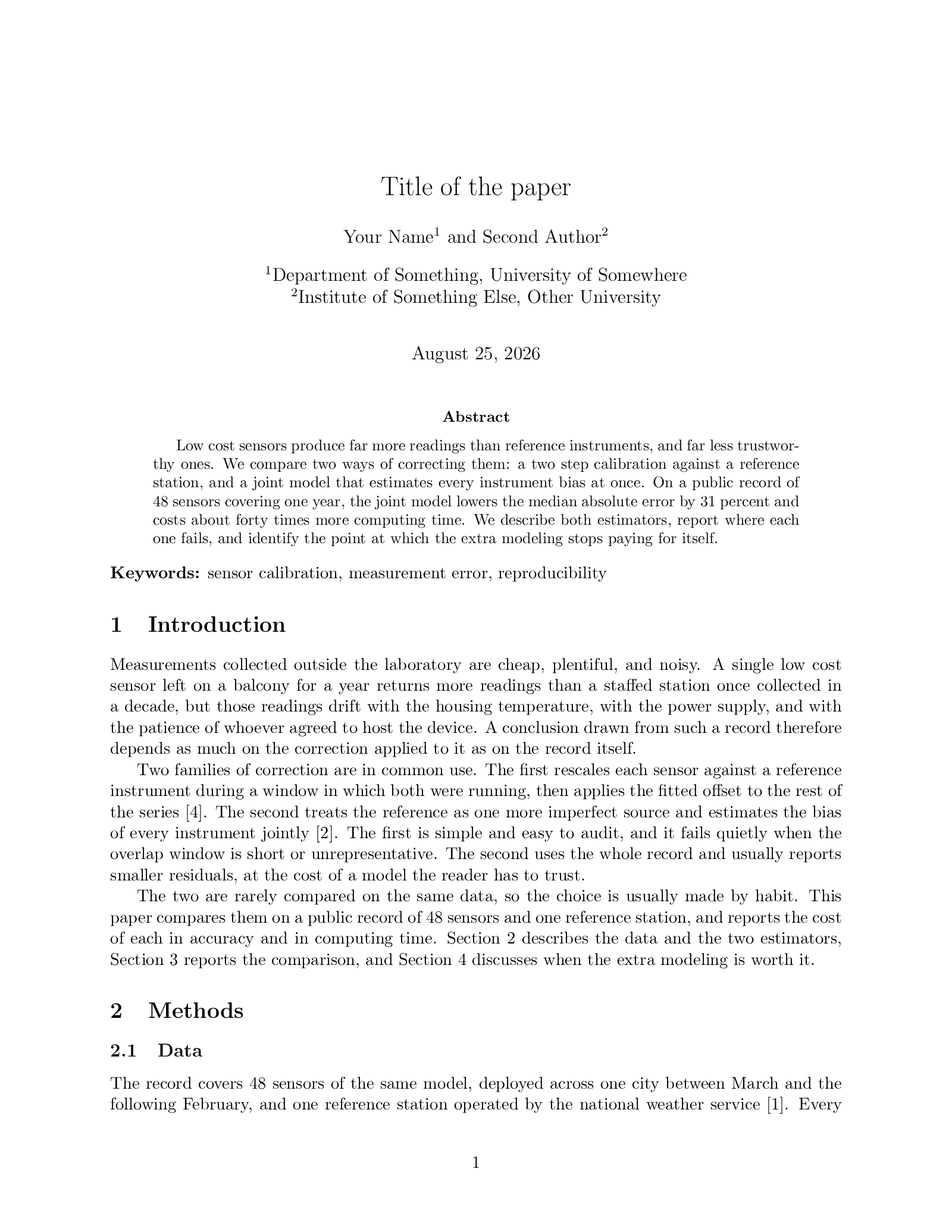
Open in LaTeX.to Download all files (zip)
Files:
main.tex
% !BIB program = bibtex
\documentclass[11pt]{article}

% Margins. Remove this line for the class defaults.
\usepackage[margin=2.5cm]{geometry}

\usepackage{amsmath}
\usepackage{amssymb}
\usepackage{booktabs}
\usepackage{tikz}
\usetikzlibrary{arrows.meta,positioning}
\usepackage{authblk}
\usepackage[numbers]{natbib}
\usepackage{hyperref} % keep hyperref last

\title{Title of the paper}

% One \author per person, one \affil per institution, matched by number.
\author[1]{Your Name}
\author[2]{Second Author}
\affil[1]{Department of Something, University of Somewhere}
\affil[2]{Institute of Something Else, Other University}

\date{\today}

\begin{document}
\maketitle

\begin{abstract}
% One paragraph: the problem, what you did, what you found.
Low cost sensors produce far more readings than reference instruments, and far
less trustworthy ones. We compare two ways of correcting them: a two step
calibration against a reference station, and a joint model that estimates every
instrument bias at once. On a public record of 48 sensors covering one year,
the joint model lowers the median absolute error by 31 percent and costs about
forty times more computing time. We describe both estimators, report where each
one fails, and identify the point at which the extra modeling stops paying for
itself.
\end{abstract}

\noindent\textbf{Keywords:} sensor calibration, measurement error, reproducibility

\section{Introduction}
\label{sec:introduction}
% What the problem is, why it matters, what this paper adds.
Measurements collected outside the laboratory are cheap, plentiful, and noisy.
A single low cost sensor left on a balcony for a year returns more readings
than a staffed station once collected in a decade, but those readings drift
with the housing temperature, with the power supply, and with the patience of
whoever agreed to host the device. A conclusion drawn from such a record
therefore depends as much on the correction applied to it as on the record
itself.

Two families of correction are in common use. The first rescales each sensor
against a reference instrument during a window in which both were running, then
applies the fitted offset to the rest of the series \cite{smith2021}. The
second treats the reference as one more imperfect source and estimates the bias
of every instrument jointly \cite{lopez2019}. The first is simple and easy to
audit, and it fails quietly when the overlap window is short or unrepresentative.
The second uses the whole record and usually reports smaller residuals, at the
cost of a model the reader has to trust.

The two are rarely compared on the same data, so the choice is usually made by
habit. This paper compares them on a public record of 48 sensors and one
reference station, and reports the cost of each in accuracy and in computing
time. Section~\ref{sec:methods} describes the data and the two estimators,
Section~\ref{sec:results} reports the comparison, and
Section~\ref{sec:discussion} discusses when the extra modeling is worth it.

\section{Methods}
\label{sec:methods}

\subsection{Data}
The record covers 48 sensors of the same model, deployed across one city
between March and the following February, and one reference station operated by
the national weather service \cite{hernandez2020}. Every device reports once a
minute; we averaged to hourly means and discarded hours in which a device
reported fewer than 40 readings. That left 361{,}000 sensor hours, of which 6.2
percent overlap the reference station.

Figure~\ref{fig:pipeline} shows the three stages the data passes through. Each
stage writes its output to disk, so a change to the bias model does not force
the raw readings to be parsed again. The code and the intermediate files are
archived with the paper.

\begin{figure}[t]
  \centering
  \begin{tikzpicture}[
    node distance=6mm,
    stage/.style={draw, rounded corners, minimum width=20mm,
                  minimum height=9mm, align=center, font=\small}
  ]
    \node[stage] (raw) {Raw\\readings};
    \node[stage, right=of raw] (fit) {Bias\\model};
    \node[stage, right=of fit] (out) {Corrected\\series};
    \draw[-{Stealth}] (raw) -- (fit);
    \draw[-{Stealth}] (fit) -- (out);
  \end{tikzpicture}
  \caption{The three stages of the pipeline. Each stage is a separate program
  reading and writing plain text, so any one of them can be replaced without
  rerunning the others.}
  \label{fig:pipeline}
\end{figure}

\subsection{Estimators}
Write $y_{it}$ for the reading of sensor $i$ at hour $t$, $\mu_t$ for the true
value, and $b_i$ for the bias of the sensor. Both estimators assume the same
model,
\begin{equation}
  \label{eq:model}
  y_{it} = \mu_t + b_i + \varepsilon_{it},
  \qquad \varepsilon_{it} \sim \mathcal{N}(0, \sigma_i^2),
\end{equation}
and differ only in what they hold fixed. The two step estimator takes $\mu_t$
from the reference station wherever the two overlap, solves
Equation~\eqref{eq:model} for $b_i$ on that subset, and subtracts the result
everywhere. The joint estimator treats $\mu_t$ and every $b_i$ as unknown and
maximizes the likelihood over all of them at once, with the reference station
entered as a sensor whose $\sigma_i$ is known to be small.

\section{Results}
\label{sec:results}
Table~\ref{tab:comparison} reports the median absolute error against a set of
held out reference hours that neither estimator saw. Correcting the readings at
all matters more than the choice of estimator: both methods remove most of the
error, and the joint model then removes about a third of what is left.

\begin{table}[t]
  \centering
  \caption{Median absolute error and running time for the two estimators, over
  48 sensors and one year of hourly readings.}
  \label{tab:comparison}
  \begin{tabular}{lrr}
    \toprule
    Estimator    & Median error (K) & Time (s) \\
    \midrule
    Uncorrected  & 1.42 & 0 \\
    Two step     & 0.61 & 3 \\
    Joint model  & 0.42 & 128 \\
    \bottomrule
  \end{tabular}
\end{table}

The gap is not evenly spread. For the 31 sensors whose overlap with the
reference exceeds one week, the two estimators agree to within 0.05 K. The
remaining 17 sensors carry almost all of the difference, and 4 of them are
corrected in the wrong direction by the two step method.

\section{Discussion}
\label{sec:discussion}
The joint model earns its cost only where the overlap window is short. That is
a useful rule, because the length of the overlap is known before either
estimator is run. A deployment that can afford to leave every device beside the
reference for a week has little to gain from the heavier method, while a
deployment that recruits hosts as it goes has a great deal to gain.

The main threat to this conclusion is that both estimators assume a bias that
does not change over the year, and Equation~\eqref{eq:model} has no term for
drift. Earlier work reports drift of about 0.1 K per year for this sensor
family \cite{okafor2022}, small next to the errors in
Table~\ref{tab:comparison} but not negligible for a longer deployment.

\section{Conclusion}
Joint estimation of sensor bias is worth its cost when calibration overlaps are
short, and close to pointless when they are long. Both estimators, the data,
and the held out hours used here are archived so that a third method can be
compared on the same terms.

\bibliographystyle{plainnat}
\bibliography{references}

\end{document}
references.bib
% One entry per reference. The key (smith2021) is what you pass to \cite.
@article{smith2021,
  author  = {Alice Smith and Bharat Rao},
  title   = {Two step calibration of low cost temperature sensors},
  journal = {Journal of Atmospheric Measurement},
  volume  = {14},
  number  = {3},
  pages   = {201-218},
  year    = {2021}
}

@inproceedings{lopez2019,
  author    = {Marta Lopez and Yusuf Demir},
  title     = {Joint estimation of instrument bias in dense sensor networks},
  booktitle = {Proceedings of the Conference on Environmental Sensing},
  pages     = {77-86},
  year      = {2019}
}

@article{hernandez2020,
  author  = {Paulo Hernandez},
  title   = {A public record of urban temperature at street level},
  journal = {Data in Environmental Science},
  volume  = {6},
  pages   = {45-59},
  year    = {2020}
}

@article{okafor2022,
  author  = {Ngozi Okafor and Lars Vogel},
  title   = {Long term drift in inexpensive temperature sensors},
  journal = {Sensors and Actuators},
  volume  = {338},
  pages   = {112-124},
  year    = {2022}
}
How to use this template
Everything runs in your browser: nothing to install, no login, no compile timeout.
- Click Open in LaTeX.to. The template opens as a project in the Projects pane, with main.tex in the editor and its finished PDF in the preview.
- Click Preview, or press Ctrl+Enter (Cmd+Enter on a Mac), to compile. The preview shows the new PDF; you do not need to save first.
- If the compile fails, the Console pane opens with the LaTeX log. The first error in it says what went wrong and on which line.
- To add an image, a .bib file or another .tex file, open the project's menu (the three dots next to its name in the Projects pane) and choose Upload file or New file.
- The arrow next to Preview has Download PDF. Ctrl+S saves your edits, and the project stays in your browser on this device.
How to add a reference
References come from references.bib, and BibTeX runs by itself when you compile.
- Click
references.bibin the Projects pane and add an entry; copy an existing one and change the key, authors, title, journal and year. - Cite it with
\cite{key}for a number in brackets, or\citet{key}for "Author et al. [3]" in the sentence. - The list at the end is sorted by author and updates on the next compile.
How to use two columns
The file is one column, and the two column look of a journal paper is one class option away.
- Change the
\documentclassline to\documentclass[11pt,twocolumn]{article}. - Put a figure or table that is wider than one column in
figure*ortable*; it then spans the page. - The abstract prints as a plain section inside the left column, not centered across the page.
- Split a long equation over two lines with the
multlineenvironment, since a column is narrow.
How to add an author
Authors and affiliations are matched by number.
- Add
\author[3]{Third Author}below the second author line. - If they are at a new institution, add
\affil[3]{Institute, University}; if they share an institution, use its number in the\authorline instead. - Two numbers on one author, as in
\author[1,2]{...}, list both affiliations.
More templates: ACM paper, Beamer presentation, Elsevier article, IEEE paper, Poster, Research proposal, Thesis and all templates.