LaTeX TikZ template

A LaTeX TikZ template for a document whose figures are drawn in the source: a diagram, two constructions and a plot to copy and adapt.

Open in LaTeX.to Download all files (zip)

Engine: pdfLaTeX
Bibliography: none
License: Public domain, use freely.

Files:

main.tex

Download main.tex

\documentclass[11pt,a4paper]{article}

\usepackage[T1]{fontenc}
\usepackage[margin=25mm]{geometry}
\usepackage{lmodern}
% [H] below keeps each figure where it is written instead of letting it float.
\usepackage{float}
\usepackage{tikz}
\usetikzlibrary{arrows.meta,positioning,shapes.geometric,calc,angles,quotes}
\usepackage{pgfplots}
\pgfplotsset{compat=1.18}

% Three lines to change: title, author, date.
\title{Figures Drawn in the Source}
\author{Your Name}
\date{\today}

\begin{document}
\maketitle

\section{Introduction}
Every figure in this document is written as TikZ source next to the text it
belongs to, so it uses the same fonts and the same math as the body and there
is no image file to keep in sync. Figure~\ref{fig:shapes} shows the basic
vocabulary, Figure~\ref{fig:geometry} two constructions computed by TeX,
Figure~\ref{fig:flowchart} a diagram built from named nodes, and
Figure~\ref{fig:plot} a chart drawn by \texttt{pgfplots}. Copy the one closest
to what you need and change the numbers.

\section{Shapes and paths}
Coordinates, straight lines, rectangles, circles and B\'ezier curves are the
vocabulary. The options in square brackets set colour, line width, fill and
arrow tips.

\begin{figure}[H]
\centering
\begin{tikzpicture}
% The grid and the axes. Change (4,2.5) to grow the canvas.
\draw[help lines, step=0.5] (0,0) grid (4,2.2);
\draw[->, thick] (0,0) -- (4.4,0) node[right] {$x$};
\draw[->, thick] (0,0) -- (0,2.6) node[above] {$y$};
% A colour such as blue!15 is 15 percent blue mixed with white.
\draw[fill=blue!15, draw=blue!60!black, thick] (0.5,0.5) rectangle (1.75,1.75);
\draw[fill=orange!30, draw=orange!70!black, thick] (2.6,1.25) circle (0.7);
\draw[red, very thick, dashed] (0.5,1.9) .. controls (1.5,2.7) and (2.5,0.8) .. (3.8,2.0);
\draw[-{Stealth[length=3mm]}, green!50!black, thick] (3.5,0.4) -- (1.95,1.15);
\end{tikzpicture}
\caption{A rectangle, a circle, a B\'ezier curve and an arrow on a grid.}
\label{fig:shapes}
\end{figure}

\section{Constructions computed by TeX}
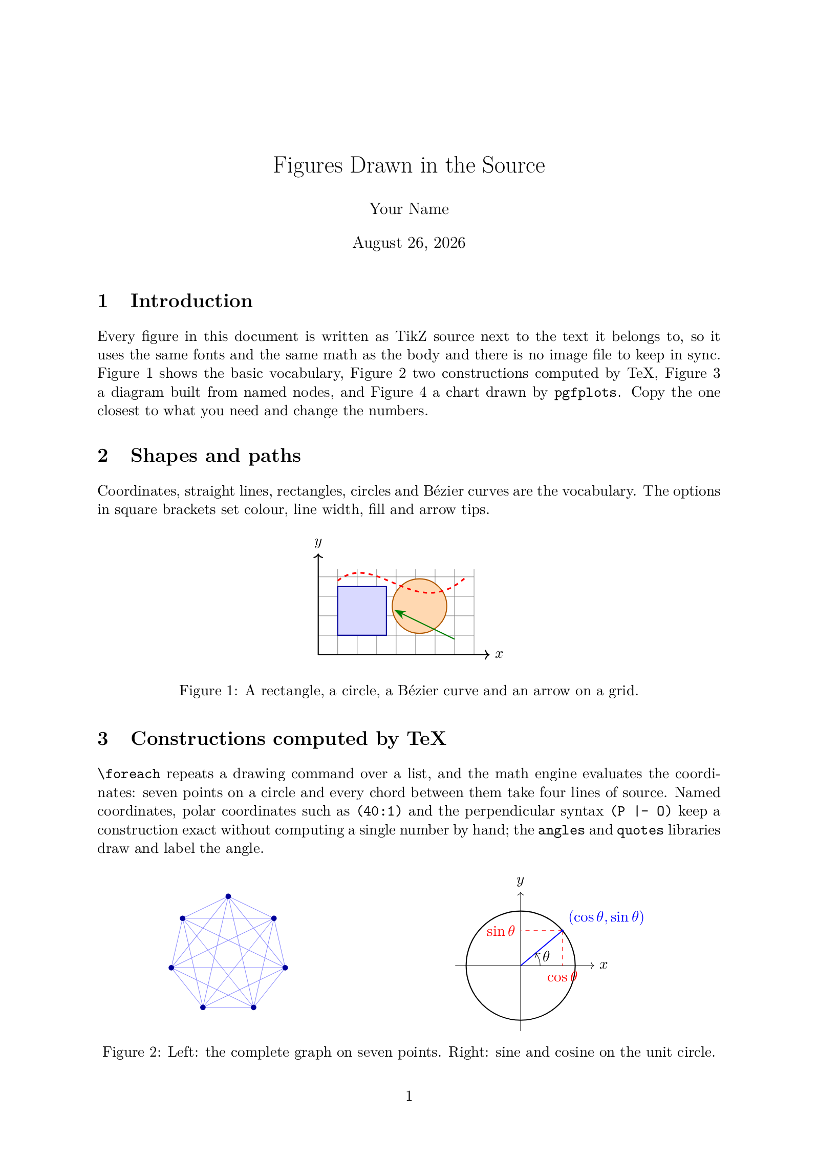
\verb|\foreach| repeats a drawing command over a list, and the math engine
evaluates the coordinates: seven points on a circle and every chord between
them take four lines of source. Named coordinates, polar coordinates such as
\texttt{(40:1)} and the perpendicular syntax \texttt{(P |- O)} keep a
construction exact without computing a single number by hand; the
\texttt{angles} and \texttt{quotes} libraries draw and label the angle.

\begin{figure}[H]
\centering
\begin{minipage}{0.42\linewidth}
\centering
\begin{tikzpicture}
% Change both 7s to draw the complete graph on another number of points.
\foreach \i in {1,...,7} {
  \coordinate (p\i) at ({90+360/7*(\i-1)}:1.5);
}
\foreach \i [evaluate=\i as \next using int(\i+1)] in {1,...,6}
  \foreach \j in {\next,...,7}
    \draw[blue!45, thin] (p\i) -- (p\j);
\foreach \i in {1,...,7}
  \fill[blue!60!black] (p\i) circle (2pt);
\end{tikzpicture}
\end{minipage}
\hfill
\begin{minipage}{0.54\linewidth}
\centering
\begin{tikzpicture}[scale=1.4]
\draw[->] (-1.2,0) -- (1.35,0) node[right] {$x$};
\draw[->] (0,-1.2) -- (0,1.35) node[above] {$y$};
\draw[thick] (0,0) circle (1);
\coordinate (O) at (0,0);
\coordinate (X) at (1,0);
% The angle: 40 degrees, radius 1.
\coordinate (P) at (40:1);
\draw[thick, blue] (O) -- (P) node[above right] {$(\cos\theta,\sin\theta)$};
\draw[dashed, red] (P) -- (P |- O) node[below] {$\cos\theta$};
\draw[dashed, red] (P) -- (P -| O) node[left] {$\sin\theta$};
\pic[draw, ->, "$\theta$", angle eccentricity=1.4, angle radius=5mm] {angle=X--O--P};
\fill[blue] (P) circle (0.6pt);
\end{tikzpicture}
\end{minipage}
\caption{Left: the complete graph on seven points. Right: sine and cosine on
the unit circle.}
\label{fig:geometry}
\end{figure}

\section{A flowchart}
A node is a shape with text inside, and the \texttt{positioning} library
places nodes relative to each other. The styles defined at the top of the
picture keep every box alike, and the arrows connect nodes by name, so moving
one box moves its arrows with it.

\begin{figure}[H]
\centering
\begin{tikzpicture}[node distance=7mm and 12mm, font=\small,
  box/.style={draw, rounded corners, fill=blue!8, minimum width=26mm,
    minimum height=8mm, align=center},
  decision/.style={diamond, draw, fill=orange!15, aspect=2, inner sep=1pt},
  arrow/.style={-{Stealth[length=2.5mm]}, thick}]
% One line per box: the text in braces, the name in parentheses.
\node[box] (edit) {Edit \texttt{main.tex}};
\node[box, below=of edit] (compile) {Compile};
\node[decision, below=of compile] (errors) {Errors?};
\node[box, right=of errors] (fix) {Read the log,\\fix the line};
\node[box, below=of errors] (pdf) {Download the PDF};
% One line per arrow, from name to name; a node[...] in between labels it.
\draw[arrow] (edit) -- (compile);
\draw[arrow] (compile) -- (errors);
\draw[arrow] (errors) -- node[above] {yes} (fix);
\draw[arrow] (fix) |- (edit);
\draw[arrow] (errors) -- node[right] {no} (pdf);
\end{tikzpicture}
\caption{The edit, compile and fix loop as a flowchart.}
\label{fig:flowchart}
\end{figure}

\section{A plot}
\texttt{pgfplots} builds on TikZ and draws the axes, ticks, grid and legend
from a function or from a list of numbers. The curves in
Figure~\ref{fig:plot} are evaluated by TeX at compile time.

\begin{figure}[H]
\centering
\begin{tikzpicture}
\begin{axis}[width=0.85\linewidth, height=58mm, domain=0:4*pi, samples=200,
  xlabel={$x$}, ylabel={$y$}, grid=major, legend pos=north east,
  xtick={0,3.1416,6.2832,9.4248,12.566},
  xticklabels={$0$,$\pi$,$2\pi$,$3\pi$,$4\pi$}]
% One \addplot per curve. Angles are in degrees, hence deg(x).
\addplot[blue, thick] {sin(deg(x))};
\addplot[red, thick] {exp(-0.25*x)*cos(deg(x))};
% One legend entry per \addplot, in the same order.
\legend{$\sin x$, $e^{-x/4}\cos x$}
\end{axis}
\end{tikzpicture}
\caption{Two functions on one axis, with a grid and a legend.}
\label{fig:plot}
\end{figure}

\end{document}

How to use this template

Everything runs in your browser: nothing to install, no login, no compile timeout.

Click Open in LaTeX.to. The template opens as a project in the Projects pane, with main.tex in the editor and its finished PDF in the preview.
Replace the placeholders, such as Your Name, with your own text. The % comments in the files mark the places to edit.
Click Preview, or press Ctrl+Enter (Cmd+Enter on a Mac), to compile. The preview shows the new PDF; you do not need to save first.
If the compile fails, the Console pane opens with the LaTeX log. The first error in it says what went wrong and on which line.
To add an image, a .bib file or another .tex file, open the project's menu (the three dots next to its name in the Projects pane) and choose Upload file or New file.
The arrow next to Preview has Download PDF. Ctrl+S saves your edits, and the project stays in your browser on this device.

How to add a figure of your own

Every picture sits in a figure environment, so a new one gets a number, a caption and a reference like the others.

Copy the block from \begin{figure}[H] to \end{figure} and paste it where the new figure belongs.
Replace everything between \begin{tikzpicture} and \end{tikzpicture} with your own drawing commands.
Change the \caption{...} text and give the \label{fig:...} line a new name.
Refer to it in the text with Figure~\ref{fig:name}; the numbers follow on the next compile.

How to change colours and lines

The options in square brackets after \draw and \node set how a path looks.

A colour such as blue!15 is 15 percent blue mixed with white; blue!60!black is 60 percent blue mixed with black.
thin, thick and very thick set the line width, dashed and dotted the pattern.
-{Stealth[length=3mm]} puts an arrow tip at the end of a path; <-> puts one at both ends.
In the flowchart, the box/.style={...} line at the top of the picture changes every box at once.

How to save one figure as an image

A figure is often needed on its own, for a slide or a web page.

Compile, then open the Preview menu and choose Download image.
Drag a rectangle around the figure on the page and download the PNG.

More templates: Article, Book, Letter and all templates.