LaTeX lab report template

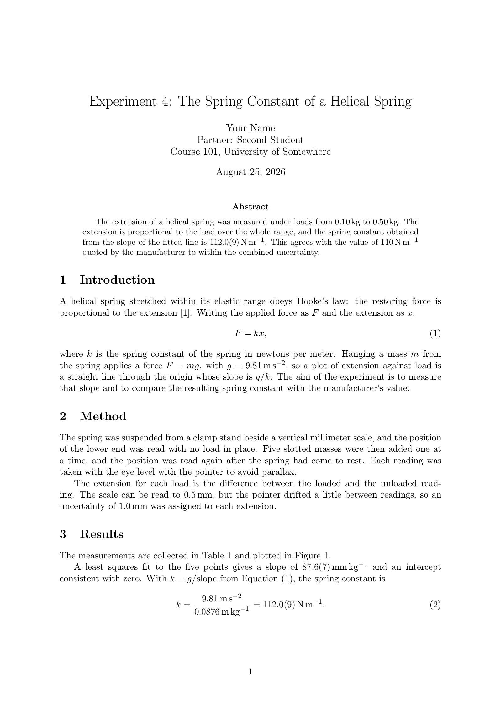
A LaTeX lab report template for a physics or chemistry write-up, with a measurements table and a plot.

Open in LaTeX.to Download all files (zip)

Engine: pdfLaTeX
Bibliography: none
License: Public domain, use freely.

Files:

main.tex

\documentclass[11pt,a4paper]{article}

\usepackage[margin=2.5cm]{geometry}
\usepackage{amsmath}
\usepackage{booktabs}
\usepackage{siunitx}   % units and uncertainties: \qty, \unit, S columns
\usepackage{graphicx}  % for \includegraphics once you upload a photo
\usepackage{pgfplots}  % the plot in the Results section
\pgfplotsset{compat=1.18}
\usepackage{hyperref}  % keep hyperref last

% Experiment, your name, your lab partner, the course.
\title{Experiment 4: The Spring Constant of a Helical Spring}
\author{Your Name \\ Partner: Second Student \\ Course 101, University of Somewhere}
\date{\today}

\begin{document}
\maketitle

\begin{abstract}
The extension of a helical spring was measured under loads from
\qty{0.10}{\kilogram} to \qty{0.50}{\kilogram}. The extension is proportional
to the load over the whole range, and the spring constant obtained from the
slope of the fitted line is \qty{112.0(9)}{\newton\per\meter}. This agrees
with the value of \qty{110}{\newton\per\meter} quoted by the manufacturer to
within the combined uncertainty.
\end{abstract}

\section{Introduction}

A helical spring stretched within its elastic range obeys Hooke's law: the
restoring force is proportional to the extension~\cite{halliday2018}. Writing
the applied force as $F$ and the extension as $x$,
\begin{equation} \label{eq:hooke}
  F = k x ,
\end{equation}
where $k$ is the spring constant of the spring in newtons per meter. Hanging a
mass $m$ from the spring applies a force $F = mg$, with
$g = \qty{9.81}{\meter\per\second\squared}$, so a plot of extension against
load is a straight line through the origin whose slope is $g/k$. The aim of
the experiment is to measure that slope and to compare the resulting spring
constant with the manufacturer's value.

\section{Method}

The spring was suspended from a clamp stand beside a vertical millimeter
scale, and the position of the lower end was read with no load in place. Five
slotted masses were then added one at a time, and the position was read again
after the spring had come to rest. Each reading was taken with the eye level
with the pointer to avoid parallax.

The extension for each load is the difference between the loaded and the
unloaded reading. The scale can be read to \qty{0.5}{\milli\meter}, but the
pointer drifted a little between readings, so an uncertainty of
\qty{1.0}{\milli\meter} was assigned to each extension.

\section{Results}

The measurements are collected in Table~\ref{tab:extension} and plotted in
Figure~\ref{fig:extension}.

\begin{table}[htbp]
  \centering
  \caption{Extension of the spring for each load.}
  \label{tab:extension}
  \begin{tabular}{
      S[table-format=1.2]
      S[table-format=2.1]
      S[table-format=1.1]
    }
    \toprule
    {Load $m$ (\unit{\kilogram})} & {Extension $x$ (\unit{\milli\meter})} &
      {Uncertainty (\unit{\milli\meter})} \\
    \midrule
    0.10 &  8.9 & 1.0 \\
    0.20 & 17.3 & 1.0 \\
    0.30 & 26.6 & 1.0 \\
    0.40 & 34.8 & 1.0 \\
    0.50 & 44.1 & 1.0 \\
    \bottomrule
  \end{tabular}
\end{table}

\begin{figure}[htbp]
  \centering
  \begin{tikzpicture}
    \begin{axis}[
        width=0.8\linewidth,
        height=6.5cm,
        xlabel={Load $m$ (kg)},
        ylabel={Extension $x$ (mm)},
        xmin=0, xmax=0.55,
        ymin=0, ymax=50,
        xtick={0, 0.1, 0.2, 0.3, 0.4, 0.5},
        grid=both,
        legend pos=south east,
      ]
      % Replace these rows with your own measurements.
      \addplot+[only marks, error bars/.cd, y dir=both, y explicit]
        table[x=load, y=ext, y error=err] {
          load  ext   err
          0.10   8.9  1.0
          0.20  17.3  1.0
          0.30  26.6  1.0
          0.40  34.8  1.0
          0.50  44.1  1.0
        };
      \addlegendentry{Measured}
      \addplot[thick, domain=0:0.55, samples=2] {87.6*x + 0.1};
      \addlegendentry{Fitted line}
    \end{axis}
  \end{tikzpicture}
  \caption{Extension against load, with the fitted straight line.}
  \label{fig:extension}
\end{figure}

A least squares fit to the five points gives a slope of
\qty{87.6(7)}{\milli\meter\per\kilogram} and an intercept consistent with
zero. With $k = g / \text{slope}$ from Equation~\eqref{eq:hooke}, the spring
constant is
\begin{equation} \label{eq:result}
  k = \frac{\qty{9.81}{\meter\per\second\squared}}
           {\qty{0.0876}{\meter\per\kilogram}}
    = \qty{112.0(9)}{\newton\per\meter} .
\end{equation}

\section{Discussion}

The points lie on the fitted line to within their error bars, so the spring
stayed inside its elastic range for every load used. The result in
Equation~\eqref{eq:result} is \qty{1.8}{\percent} above the manufacturer's
value of \qty{110}{\newton\per\meter}, a difference of about twice the
uncertainty of the fit, which suggests a small systematic effect rather than
random error.

The most likely source is the mass of the spring itself, which is not included
in the load but does stretch the upper coils. Reading the scale by eye is the
second source: a parallax error of one millimeter on the unloaded reading
shifts every extension by the same amount, which moves the intercept but not
the slope, so it does not explain the difference. Averaging three readings per
load and correcting for the mass of the spring would tighten the result.

\section{Conclusion}

The extension of the spring is proportional to the load between
\qty{0.10}{\kilogram} and \qty{0.50}{\kilogram}, as Hooke's law predicts. The
spring constant measured from the slope is
\qty{112.0(9)}{\newton\per\meter}, close to the quoted value of
\qty{110}{\newton\per\meter}. The method described by
Taylor~\cite{taylor1997} was used to propagate the uncertainties.

\begin{thebibliography}{9}

\bibitem{halliday2018}
  David Halliday, Robert Resnick and Jearl Walker,
  \emph{Fundamentals of Physics}, 11th edition, Wiley, 2018.

\bibitem{taylor1997}
  John R. Taylor,
  \emph{An Introduction to Error Analysis}, 2nd edition,
  University Science Books, 1997.

\end{thebibliography}

\end{document}

How to use this template

Everything runs in your browser: nothing to install, no login, no compile timeout.

Click Open in LaTeX.to. The template opens as a project in the Projects pane, with main.tex in the editor and its finished PDF in the preview.
Replace the placeholders, such as Your Name, with your own text. The % comments in the files mark the places to edit.
Click Preview, or press Ctrl+Enter (Cmd+Enter on a Mac), to compile. The preview shows the new PDF; you do not need to save first.
If the compile fails, the Console pane opens with the LaTeX log. The first error in it says what went wrong and on which line.
To add an image, a .bib file or another .tex file, open the project's menu (the three dots next to its name in the Projects pane) and choose Upload file or New file.
The arrow next to Preview has Download PDF. Ctrl+S saves your edits, and the project stays in your browser on this device.

How to enter your own measurements

The table and the plot each hold a copy of the numbers, so change both.

In the tabular under \label{tab:extension}, replace the five rows like 0.10 & 8.9 & 1.0 \\ with your own, one row per measurement, keeping the & between the columns and the \\ at the end.
In the plot, replace the rows after load ext err with the same numbers, separated by spaces.
The S columns line the decimal points up; table-format=2.1 means two digits before the point and one after, so widen it if your numbers are bigger.
Adjust xmax, ymax and xtick in the axis options to the range of your data.
Put your own slope and intercept into the line \addplot[thick, domain=0:0.55, samples=2] {87.6*x + 0.1};, which draws the fitted line.

How to add a photo of the setup

The graphicx package is already loaded, so a photo is an upload and a few lines.

Open the project's menu in the Projects pane, choose Upload file and pick the image (PNG, JPG or PDF).
Where the figure belongs, add \begin{figure}[htbp] \centering \includegraphics[width=0.7\linewidth]{setup.jpg} \caption{The experimental setup.} \label{fig:setup} \end{figure}, one command per line.
Refer to it in the text with Figure~\ref{fig:setup}; the number follows the order of the figures.

More templates: Cheat sheet, Homework, Report and all templates.